Sinkpath

Thermal and hydraulic modeling

Junction to ambient, in one model.

Sinkpath predicts chip temperature, pressure budgets, facility efficiency and device reliability for liquid-cooled datacenters. Cold plate and immersion, single phase and two phase, from geometry and operating conditions. Every branch is checked against published measurements.

Beta model coming out soon

In active development. Beta access opens as the remaining validation branches close.

Temperature cascade

Worked example: single-phase cold plate, 1 kW device, chillered plant
AMBIENT 35.0 °C Package Cold plate Caloric CDU approach Compressor lift Heat rejection CHIPJunction59.4 °C PACKAGECase49.4 °C COOLERPlate wall37.4 °C TCSCoolant in35.0 °C CDUFWS supply30.0 °C CHILLERCondenser42.0 °C PLANTAmbient35.0 °C

Heat leaves the die and crosses every interface in turn. Each leg is a resistance the model computes rather than assumes, and each node is a temperature it reports. The compressor is the one leg that runs uphill, which is why the plant is where facility power is won or lost. The same solver returns the pressure budget along the identical path.

The same cascade, at package level

Lidded stack, single-phase cold plate, 1 kW device
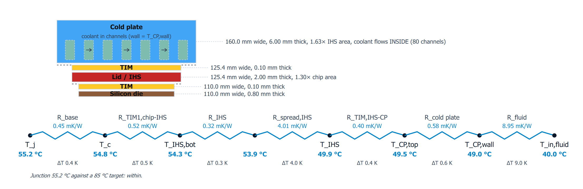
Package cross section showing silicon die, TIM, lid or IHS, second TIM and cold plate with their widths and thicknesses, above a resistance network from junction at 55.2 degrees Celsius through case, IHS bottom, IHS, cold plate top and cold plate wall to fluid inlet at 40.0 degrees Celsius, with the resistance of each leg in milli kelvin per watt.
(Not the same case as the system cascade plotted above.) Zoom in on the first leg of the cascade and the same treatment applies: every layer of the stack is a resistance with a temperature either side of it, drawn from the geometry you entered rather than lumped into a single junction-to-case figure. Two legs carry most of the budget here, spreading through the lid at 4.01 mK/W and the fluid itself at 8.95 mK/W, and everything else sits under half a kelvin. Splitting the stack out is what makes that visible.
Levels

Seven control volumes, one continuous solve.

Each level owns its own boundary conditions and the geometry of what sits inside it. Change a channel width and the effect travels all the way out to plant power, then comes back as a junction temperature.

01PackageDie, lid or bare die, TIM stack, spreading and conduction. Or a measured junction-to-case resistance entered as a single value, a flow curve, a polynomial or an itemized series.
02ServerCold plates or immersion heat sinks per chip section, heterogeneous loads, quick disconnects, and the branch hydraulics along each flow path.
03RackManifolds, series and parallel composition, and pairing rules that block incompatible hardware rather than warning about it.
04TCSThe technology cooling system loop. Single phase or two phase, cold plate or immersion, with the fluid library and design rise that set the caloric floor.
05CDUEffectiveness NTU on liquid exchangers, condensing form when the secondary side boils, and off-rating UA scaling from the vendor rating point.
06Hall and facility waterRoom level aggregation, facility water supply and return, glycol fraction, loop pressure and treatment.
07PlantHeat rejection and economizer staging, sized against the climate the hall actually sits in. Returns TUE, PUE and WUE.
Sinkpath level selection screen. Five checkable cards, all selected: Datacenter for total facility-level power modeling, Server Room for room and rack or cabinet layout, Rack or Cabinet for enclosure-level configuration, Server for server-power level configuration, and Chip for heat sink, TIM and fin-level thermal configuration.
You choose how far down the stack to go before anything is entered, and that choice sets which parameters the rest of the wizard asks for. A facility study and a fin-level study are the same solve run to different depths, so nothing has to be re-entered to move between them.
Plant

Pick the rejection path, then let the weather decide the duty.

The plant is where most of the argument about a cooling design actually happens, so it is modeled as a choice rather than a constant. Each option carries its own approach behaviour, its own parasitic power and its own water draw, and every one of them moves with wet bulb and dry bulb through the year.

Water-cooled chillerCompressor lift against a condenser loop, with part load behaviour and a lift that follows condenser water temperature.
Air-cooled chillerNo tower, no water draw, and a condensing temperature tied directly to dry bulb. Usually the PUE penalty and the WUE win at the same time.
Open cooling towerWet bulb approach, evaporative loss, drift and blowdown carried explicitly into the water balance.
Closed circuit towerIsolated process loop with an evaporative outer circuit, for sites that want tower performance without exposing the facility water.
Dry coolerDry bulb approach, zero water. The reference case for warm water designs that never need a compressor.
Adiabatic coolerDry most of the year, pre-cooled on the hot hours only. Water is spent where it buys the most approach.
Heat pumpLift taken deliberately rather than reluctantly, to raise return water to a temperature something else can use.
GeothermalGround or groundwater loop as a stable low temperature sink, sized on soil conditions rather than air.
Radiative sky and cool roofLongwave rejection to the sky and surface treatments, both strongly climate dependent and both reported as hours rather than as a rating.

Economizer duty, by climate.

Free cooling is not a yes or no answer. For a given supply temperature, a site spends the year moving between full economizer, partial economizer with trim, and full mechanical cooling, and the split is what actually sets annual energy and water. Sinkpath runs the design point and then runs the year, and reports both.

Full economizer hoursAmbient cold enough that the compressor stays off and the approach alone carries the load.
Partial with mechanical trimEconomizer takes what it can, the chiller makes up the difference, and the lift is only as large as the shortfall.
Full mechanicalDesign day behaviour, which sets equipment size even when it represents a small fraction of the year.

The same site and the same supply temperature, run twice with only the rejection path changed, shows how much the choice of sink is worth. Austin, Texas is a useful test because it is mild enough that dry rejection looks viable on an annual average and hot enough that the average hides the problem.

Full year economizer split for Austin, Texas with a dry cooler. Stacked daily bars showing 5,178 hours of full free cooling concentrated in winter, 2,299 partial hours through the summer, and the remainder chiller-only. Below it, economizer duty across July 15 rises to about 85 percent overnight and falls to zero from late morning to evening.
Dry economizer, ambient air. Winter runs at full free cooling almost continuously, but from June to September the day splits: the compressor stays off overnight and comes on through the afternoon. 5,178 hours are fully free and 2,299 are partial, leaving the balance of the year on mechanical cooling outright. The July 15 trace is the shape that matters, since duty falls to zero across the entire afternoon peak.
Full year economizer split for Austin, Texas with a wet economizer. Stacked daily bars showing all 8,760 hours of the year at full free cooling, with no partial and no chiller-only hours. Below it, economizer duty across July 15 holds flat at 100 percent for all 24 hours.
Wet economizer, cooling tower or adiabatic. The wet bulb approach carries the load for all 8,760 hours, including the July afternoon that defeats the dry case, so the compressor never runs. The trade is water, which is why WUE is reported next to PUE rather than after it: this result costs evaporation, drift and blowdown, and the dry case costs none.

Raising facility water supply by a few degrees usually moves a site between these bands more than any component swap does. That trade is the whole point of running the annual split next to the design point instead of after it.

And the case with no ambient at all.

Every option above ends by handing heat to air or to water. In orbit there is neither, and radiation to deep space is the only way out, so the terms that set the design change completely: radiator area and emissivity, view factors to the sun and to the earth, the sink temperature the surface actually sees, and the eclipse cycle of the orbit itself. Sinkpath treats this as a rejection stage like any other, which means an orbital datacenter is solved on the same junction to ambient cascade as a terrestrial one and the two can be compared on the same metrics rather than by analogy.

Schematic of a technology cooling system loop. TCS fluid enters a chip package cooled by direct-to-chip microchannels, returns through a filter, sensors and instrumentation, and a pump into a CDU. Two alternative rejection branches are drawn: (a) in space, the CDU feeds deep-space facing radiators through a second pump; (b) on Earth, the CDU feeds a dry chiller or cooling tower.
Everything upstream of the CDU is the same loop in both cases: the same package, the same microchannels, the same filter, instrumentation and pump. Only the rejection branch differs, which is the reason an orbital case can be run on the terrestrial cascade rather than as a separate model.
Orbital geometry for radiative rejection. Solar photovoltaic panels face the sun with normal vector n-PV, connected to the computational space and then to a cooling radiator whose two faces carry normals plus and minus n-rad, both at 90 degrees to the sun and Earth directions. Below, the Earth subtends a cone of half angle rho equals arcsin of Earth radius over Earth radius plus altitude h, with the nadir direction and the orbital frame of radial, tangential velocity and orbit normal unit vectors marked.
What replaces wet bulb approach in orbit. The radiator sees the sun on one side and the earth through a cone that closes as altitude rises, so orientation, altitude and the two face normals set the sink temperature the way ambient air does on the ground. Both faces are accounted separately, since a surface pointed at the earth and one pointed at deep space are not the same radiator.
Metrics

The efficiency numbers, computed rather than quoted.

Each of these comes out of the same solve, so they move together when you change something. PUE on its own hides too much, which is why TUE leads here.

TUETotal power usage effectivenessFacility power and the cooling power spent inside the IT equipment itself, counted together. Fans and on-board pumps are cooling energy no matter which side of the rack door they sit on, and TUE is the only one of these that says so.
PUEPower usage effectivenessTotal facility power over IT power, reported at the design point and as an annualized value across the economizer split.
EREEnergy reuse effectivenessCredit for heat actually exported and used elsewhere, which is where the heat pump option stops being a penalty and starts being the reason for the design.
WUEWater usage effectivenessLitres per kilowatt hour, built from evaporation, drift and blowdown rather than from a rule of thumb. Goes to zero on the dry options, which is the trade worth seeing next to PUE.
CUECarbon usage effectivenessCarbon per unit of IT energy, following the grid the site is actually on rather than a national average.
Libraries

Real hardware, not placeholder properties.

A model is only as good as what you can put into it, so these ship with the tool.

65 and countingMaterialsConventional and exotic, including the high conductivity substrates and advanced interface materials that only matter once flux gets high enough to notice them.
8Vendor serversReal chassis definitions with their published thermal and flow characteristics, rather than a generic rack unit.
10NVIDIA, AMD and Intel devicesPackage geometry, power and junction limits for current accelerators and CPUs, so a comparison starts from the device you are actually deploying.
3Immersion tanksTanks with the server configurations that go in them, since neither one means much without the other.
71Working fluidsWater and glycol mixtures, dielectrics and refrigerants, with temperature dependent properties rather than single point values.
27 and countingClimatesHourly weather for the economizer split, so the annual answer belongs to the site rather than to a category.
And these are only the defaults

Every one of these libraries is a starting point, not a boundary. Build and test your own materials, coolants and working fluids, define a climate that is not on the list, and enter your own racks, chassis and devices. If the thing you want to model does not exist yet, that is usually the reason you are modeling it.

Hydraulics

Pressure is modeled, not assumed.

Most thermal tools stop at temperature and let pump power in through a fixed allowance. Sinkpath derives the circuit from architecture and technology, then solves it: one cold plate and one connector pair per chip section at that section's own flow, pipes and manifolds sized to a design velocity, fixed bore components scaling as flow squared.

Six pressure drop model classes are available per component, from a fixed value to a fitted polynomial, a vendor table or Darcy friction. Components you have not characterized report as unmodeled instead of quietly contributing zero.
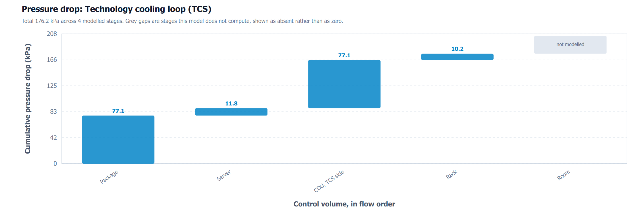
Waterfall chart of cumulative pressure drop across the technology cooling loop. Package 77.1 kPa, server 11.8 kPa, CDU TCS side 77.1 kPa, rack 10.2 kPa, room shown as not modelled. Total 176.2 kPa across four modelled stages.
Cumulative pressure drop along the technology cooling loop, in flow order. Stages the model does not compute are drawn as grey gaps rather than as zero, so an incomplete budget reads as incomplete.
Reliability

Temperature is a lifetime, not just a limit.

A design that passes at the junction temperature limit and a design that sits ten degrees below it are not equivalent, and a pass or fail verdict hides the difference. Sinkpath reports the thermal margin at every node and carries it through to device life, so a cooling choice can be argued on expected reliability rather than on headroom alone.

The same treatment applies to the plant. Approach temperatures, economizer hours and compressor lift all move with the weather, so the annual mode split is reported alongside the design point rather than in place of it.

Validation

One algorithm, checked branch by branch.

The same generic solver runs every case, with no per paper calibration and no fitted constants. Each benchmark states which values were fed and which were predicted, shows the substituted arithmetic step by step, and reports error per row with a group RMSE. Falsification cases run alongside: deliberately wrong modeling assumptions are checked to confirm they miss by margins the correct model does not.

Some branches are finished and some are still running. The table says which is which, because a validation table that only lists wins is not a validation table.

0.064 KRMSE across 11 thermal predictions, 0.19 percent of the 33.19 K driving span
66xDiscrimination ratio, how far wrong assumptions miss against the model's own error
4Cooling technologies carried by one branching algorithm
Benchmark status
BranchReferencePredictedAgreementStatus
Single-phase cold plate Published rack level experiment, IJHMT 2026. Dry cooler plant Node ladder 85.03 / 84.03 / 73.03 / 70.60 °C, three pressure budgets, 17 quantities 0.064 K, 0.011 kPa Complete
Two-phase cold plate Published server level experiment, ITherm 2024. R1233zd(E) Case to fluid resistance 0.0174 against 0.017, exit quality 0.543 against 0.55 1.23% Complete
Two-phase cold plate, cross model Published rack level model, Appl. Sci. 2023 Condenser saturation states, pressure chain, CPU temperature 0.66%, 5.2%, 1.59 K Complete
Single-phase immersion Published single chassis experiment, ICHMT 2023. FC-40 tank Consistency lattice, property web, two independent regime probes 0.050 K, 0.04% Complete
Facility water reference LBNL warm water supply reference point Supply temperature reproduced at 45.1 °C in window Complete
Two-phase immersion Pool boiling dataset selection underway Boiling curve, vapour quality, condenser duty pending In progress
Hydraulic component library Vendor curves and published branch data Component by component pressure drop across the six model classes, and the assembled circuit against a measured branch partial In progress
Server topology and flow distribution Series and parallel chassis arrangements Flow split across parallel branches, per section rise, and the penalty of series arrangements on the last device in the path partial In progress
Chiller and heat rejection Manufacturer performance data across the plant options Part load behaviour, approach against wet and dry bulb, compressor lift and parasitic power pending In progress
Economizer annual split Hourly weather against reported site performance Hours in each mode, annualized PUE and the water balance behind WUE pending Next
Coverage

What is anchored, and what is not.

Modeling tools tend to claim every technology equally. These legs are not equally supported, so here is the honest version. An experimental anchor is the strongest claim on the list. A model anchor is weaker by construction, since a published model can be reproduced faithfully and still be wrong about the world, and it is labelled as what it is rather than folded in with the rest.

Single-phase cold plateExperimental anchor, IJHMT 2026
Two-phase cold plateExperimental and cross model anchors
Single-phase immersionExperimental anchor, ICHMT 2023
Two-phase immersionStructural only, experimental anchor pending
Air cooling, CRAH and CRACModel anchor
Rear door heat exchangerModel anchor
Interposer and through-silicon via stackModel anchor
Jet impingementBenchmarking underway
Spray coolingBenchmarking underway

Two findings from that work changed the model itself. In single-phase immersion the fluid heat up resistance belongs at the tank boundary rather than stacked on the local heat transfer coefficient, and stacking it misses by a factor of fifteen. A case to fluid resistance quoted without its reference temperature is ambiguous by up to 39 percent at low flow, so every resistance reported here names inlet, bulk mean or outlet.

Who

Built inside a thermofluidics research group.

Muhammad Usama Ph.D. Candidate, University of Texas at Austin Datacenter cooling and waste heat recovery. Author of the model and of the benchmark harnesses behind every number on this page. LinkedIn
Vaibhav Bahadur Faculty advisor, University of Texas at Austin Advises the research program behind Sinkpath and the peer reviewed work the model is built on.

Try it against your own data.

If you have a rack you have measured, send the loads, flows and geometry. The useful test is a blind one: hold back the temperatures and the pressures, and see what comes out. Beta access goes out to the people who do this first.